Observability for AI stack
Trace, monitor, and debug production AI agents and LLM-powered applications.
Natively supported frameworks and libraries
OpenAI Azure
Azure LangChain
 Hugging Face
AzureLangChainHugging FaceThe AI-native observability platform
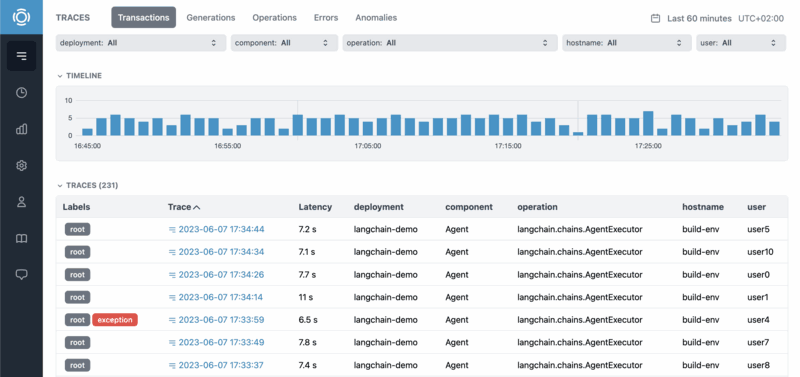
Application tracing
Trace generations, runs, and sessions with full AI context.
Scores and feedback
Evaluate any event, run, session, or user. Get notified on important feedback and issues.
Latency analysis
See latency breakdowns and distributions.
Cost tracking
Analyze model API costs for deployments, models, or users.
Error tracking
Get notified about errors and anomalies.
System monitoring
Monitor API, compute, and GPU utilization.